The Number Theoretic Transform in Kyber and Dilithium

During the last half year, I have been working on implementing the Dilithium signature scheme. Dilithium is one of the few remaining candidates in the NIST post-quantum cryptography competition. Older cryptographic signature schemes, like RSA and Ed25519, are catastrophically broken by quantum computers. Dilithium is however resistant to these quantum attacks.

My goal was to implement Dilithium efficiently on the Arduino Due, a very limited device with a Cortex-M3 core. In order to do that, I had to understand the scheme completely. Fortunately, most parts of the Dilithium scheme are not very hard to grasp, if you have some experience with vectors, matrices and rings.

However, I said most of Dilithium is not very hard. There is this one exception; one function that I think is exceptionally complicated, and I intend to clarify the hell out of it.

---

The Number Theoretic Transform (NTT) is a method that is used in Dilithium (and the related Kyber scheme) to efficiently multiply polynomials modulo some kind of prime.

It took me months to learn exactly how it works. A lot of this time was spent deciphering mathematical jargon, and trying to make the gigantic leap from theory to efficient implementation. All I needed was one good guide that explained how the NTT worked definitively and intuitively, that would have saved me so much time. I hope that this blog post may provide such a guide, and that it will help you better understand how and why the NTT works.

The number theoretic transform ¶

The number theoretic transform (NTT) is a transformation applied on rings that allows us to more efficiently compute multiplications of the elements in those rings.

The ring that is used in Dilithium is \(\mathbb{Z}_q[X]/(X^n + 1)\). This means that we are working with polynomials, with coefficients represented as integers modulo \(q\), reduced by \(X^{n} + 1\). If you know finite fields, then think of those, but without division.

Adding one element to another is done coefficient-wise. That is, if you have two polynomials

\[\begin{aligned} \mathbf{a} &= a_0 + a_1X^1 + a_2X^2 + \cdots \text{, and} \\ \mathbf{b} &= b_0 + b_1X^1 + b_2X^2 + \cdots \text{,} \\ \end{aligned}\]

then their sum \(\mathbf{c}\) is \(\mathbf{a} + \mathbf{b} = (a_0 + b_0) + (a_1 + b_1)X^1 + (a_2 + b_2)X^2 + \cdots\).

Multiplication of two polynomials is a bit more complicated. The product of two polynomials is computed by the following rule¹:

\[\mathbf{c}_k = (\mathbf{a} \cdot \mathbf{b})_k = \sum_{i + j = k} a_i b_j\]

So for every coefficient in the product, we need to do \(n\) multiplications of coefficients. Because we need to do this for \(n\) coefficients in the product, this means the multiplication complexity is \(\mathcal{O}(n^2)\). For larger values of \(n\), this becomes quite expensive!

In order to make the Dilithium scheme faster, we need to really optimize these multiplications. And that is where the NTT comes in. With the NTT, we can implement the polynomial multiplication in a super clever way. In the end, the polynomial multiplication complexity in Dilithium will only be \(\mathcal{O}(n \log n)\).

The Chinese remainder theorem ¶

Before we dive into the nasty bits of the NTT function, let me give you some background first. To understand the NTT, let us first look at the Chinese Remainder Theorem (CRT). This theorem considers a list of \(k\) numbers \(a_i\) modulo some other numbers \(m_i\). Now let \(N\) be the product of all these moduli, i.e. \(N = m_1 \cdot \cdots \cdot m_k\). The CRT says that this list of values of \(a_i\) mod \(m_i\) describes exactly one integer \(x\) mod \(N\).

For example, consider this simple system with only the two moduli \(m_1 = 11\), \(m_2 = 23\) and \(N = 11 \cdot 23 = 253\):

\[\begin{aligned} x &\equiv 3 \bmod 11 \\ x &\equiv 21 \bmod 23 \\ \end{aligned}\]

Just for fun, let us try and solve this system. :)

We are going to take the second equation and iterate over the multiples of \(23\) to see if the first equation holds. Let’s go:

\[\begin{alignedat}{3} 0 \cdot 23 + 21 &= 21 &&\stackrel{?}{\equiv} 3 \bmod 11 \hspace{10ex} &&\text{Nope.} \\ 1 \cdot 23 + 21 &= 44 &&\stackrel{?}{\equiv} 3 \bmod 11 \hspace{10ex} &&\text{Nope.} \\ 2 \cdot 23 + 21 &= 67 &&\stackrel{?}{\equiv} 3 \bmod 11 \hspace{10ex} &&\text{Nope.} \\ 3 \cdot 23 + 21 &= 90 &&\stackrel{?}{\equiv} 3 \bmod 11 \hspace{10ex} &&\text{Nope.} \\ 4 \cdot 23 + 21 &= 113 &&\stackrel{?}{\equiv} 3 \bmod 11 \hspace{10ex} &&\textbf{Yes!} \\ \end{alignedat}\]

Now we know \(x = 113 \bmod 253\)!

We can easily go back to the \(a_i\) values by just doing a modulo operation:

\[\begin{aligned} 113 \bmod 11 &= 3 \\ 113 \bmod 23 &= 21 \\ \end{aligned}\]

Of course, it is a bit tedious to do an exhaustive search every time we want to find out the value of \(x\). But don’t worry, there are more efficient algorithms that can quickly do this task for us.

Throughout this writeup we are going to use the CRT. Though before we continue, I have to mention that the CRT comes with a small print. In particular, there are some requirements for it to work:

1. We have to be working in a ring.
2. \(m_i\) values may not be equal to \(1\).
3. All \(m_i\) values have to be coprime to one another.

Residue number systems ¶

A beautiful feature of the CRT is that it allows us to construct a residue number system. That is, if we do operations on the “small” values \(a_i\), that corresponds exactly to doing the same operation to the “large” value \(x\).

For example, if we multiply the \(a_i\) values from above with \(3\), we will get:

\[\begin{alignedat}{3} x &\equiv 3 \cdot 3 &&\equiv 9 \bmod 11 \\ x &\equiv 3 \cdot 21 &&\equiv 17 \bmod 23 \\ \end{alignedat}\]

When we solve the CRT for this new system, we get \(3 \cdot 113 = 339 \equiv 86 \bmod 253\).

To show why this property is so useful, let me explain how it is used in RSA to speed up multiplications. I promise this is relevant!

Recall that in RSA, we are working modulo some very large modulus \(N\), generally around 4096 bits in size. This value \(N\) is the product of two primes \(p\) and \(q\), both of which are 2048 bits, and which are known during decryption.

Doing multiplications on a 4096-bit number \(x\) is really slow. If we would do a naive multiplication on a normal 64-bit CPU, this would involve splitting the numbers into \(64\) limbs each, and multiplying each limb with each other. That is \(64^2 = 4096\) of 64-bit multiply operations per 4096-bit multiply!

However, because \(N = p \cdot q\), it’s like RSA was made to be optimized using the CRT. Namely, if we set \(a_1 \equiv x \bmod p\) and \(a_2 \equiv x \bmod q\), we can do all computations on the smaller \(a_i\) values instead of the large \(x\) value.

Now we are only doing arithmetic on 2048-bit numbers, instead of 4096-bit numbers. For some big multiply operation, we need only \(2048\) small multiply operations². Our computation just got two times faster!³

Splitting polynomials ¶

As in RSA, the Dilithium scheme involves a lot of multiplications. The only difference is that while RSA uses large numbers, Dilithium uses a ring. The ring that is used in Dilithium is a bit unwieldy for hands-on examples, so let’s first just consider a “toy” ring.

\[R = \mathbb{Z}_q[X]/(X^n + 1) = \mathbb{Z}_{17}[X]/(X^4 + 1)\]

This ring is not used in any of the real algorithms, but let’s pretend that there exists a crypto-scheme “Di-lite-ium” that uses it. It will make our examples a lot easier to understand (and to write!). Later on, I will show that all this stuff also works on the Dilithium and Kyber rings.

We have already seen what multiplication looks like in rings:

\[\mathbf{c}_k = (\mathbf{a} \cdot \mathbf{b})_k = \sum_{i + j = k} a_i b_j\]

So for our toy ring, we have \(4 \cdot 4 = 16\) inner multiplications (\(a_i \cdot b_i\)).

---

Just like in the RSA case, we can use the CRT to reduce the number of coefficient multiplications. How would we do that? Well, let us recall what the requirements for the applying CRT were:

1. We have to be working in a ring.

Check! The \(\mathbb{Z}\) in \(\mathbb{Z}_{17}[X]/(X^4 + 1)\) stands for “ring”.

2. All \(m_i\) values have to be larger than \(1\).

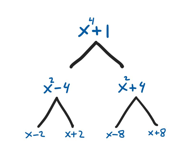
Let’s find some \(m_i\) values. We know that our modulus \(N = X^4 + 1\), and as such it is required that \(m_1 \cdot m_2 = X^4 + 1\). One possible choice of the \(m_i\) values could be:

\[\begin{aligned} m_1 &= (X^2 - 4) \\ m_2 &= (X^2 + 4) \\ \end{aligned}\]

We can quickly check that the product is indeed \(X^4 + 1\):

\[\begin{aligned} m_1m_2 &= (X^2 - 4)(X^2 + 4) \\ &= X^4 - \cancel{4X^2} + \cancel{4X^2} - 16 \\ &= X^4 - 16 \\ &\equiv X^4 + 1 \quad \checkmark \\ \end{aligned}\]

3. All \(m_i\) values have to be coprime to one another.

Yup! We can check this using the Euclidean algorithm.

All requirements for the CRT have been met! Therefore, we can express our ring using two smaller rings, with the reduction polynomials given by \(m_1\) and \(m_2\).

---

Okay, we have now rewritten our ring \(R\) as two smaller rings. Let’s call them \(R_1 = \mathbb{Z}_{17}[X]/(X^2 - 4)\) and \(R_2 = \mathbb{Z}_{17}[X]/(X^2 + 4)\). If we want to represent a polynomial \(\mathbf{a}\) modulo these smaller rings, we just use the modulo operation:

For example, in the case of \(\mathbf{a} = 2 + 7X^3\):

\[\begin{aligned} \mathbf{a} \bmod{(X^2 - 4)} &\equiv 2 + 7X^3 \\ &\equiv 2 + 7X^3 - 7X(X^2 - 4) \\ &\equiv 2 + (7 \cdot 4)X \\ &\equiv 2 + 28X \\ &\equiv 2 + 11X \\ \end{aligned}\] \[\begin{aligned} \mathbf{a} \bmod{(X^2 + 4)} &\equiv 2 + 7X^3 \\ &\equiv 2 + 7X^3 - 7X(X^2 + 4) \\ &\equiv 2 - (7 \cdot 4)X \\ &\equiv 2 - 28X \\ &\equiv 2 + 6X \\ \end{aligned}\]

We can now use these smaller degree-1 polynomials to do efficient multiplications. To multiply two sets of smaller polynomials, we only need to multiply 4 pairs of coefficients each; that is 8 multiplications in total. Just as with the RSA algorithm, we now need only half the number of multiplication operations!

Recursing down ¶

But we can go further! We can again split the \(\mathbb{Z}_{17}[X]/(X^2 - 4)\) ring into two degree-0 rings. We just have to find the other factors of \((X^2 - 4)\). We know from the last time that we are looking for two polynomials that look like \((X + \zeta)\) and \((X - \zeta)\) where \(\zeta^2 = 4\). Lucky for us, this is easy for \(4\), as we immediately see that \(\zeta = \sqrt{4} = 2\).

Now we have two new rings, namely

\[\begin{aligned} R_{1,1} &= \mathbb{Z}_{17}[X]/(X + 2)\text{ and} \\ R_{1,2} &= \mathbb{Z}_{17}[X]/(X - 2)\text{.} \\ \end{aligned}\]

which are both of degree \(0\). Indeed, only one integer is needed to store a polynomial in each of these rings. When we multiply sets of polynomials in these rings, we again need only half of the multiplication operations that we originally needed.

After splitting the large polynomial into 4 small polynomials, we have reduced the number of multiplications from \(16\) to \(4\) operations! Indeed, where \(N\) is the degree of the reduction polynomial, this transformation reduces the complexity of all the polynomial multiplications from \(\mathcal{O}(N^2)\) to \(\mathcal{O}(N)\).

Splitting Dilithium ¶

At this point, we have a method to speed up our multiplications by an enormous factor. A small recap of the steps involved:

To multiply two polynomials \(\mathbf{a}\) and \(\mathbf{b}\) into \(\mathbf{c}\):

1. Split \(\mathbf{a}\) and \(\mathbf{b}\) into \(N\) degree-0 polynomials each.
2. For \(a_i,b_i \in R_i\), compute \(c_i = a_i b_i\) using pointwise multiplication.
3. Use the Chinese remainder theorem to combine the \(c_i\) numbers back into \(\mathbf{c}\).

---

We see that this trick is very powerful in speeding up our multiplications. Let us now look at how this trick is actually applied to Dilithium.

In Dilithium, the ring that is used is more involved than the toy ring that we have seen in the previous section. It is defined by:

\[\begin{aligned} R_q &= \mathbb{Z}_q[X]/(X^{256} + 1) \end{aligned}\]

We are going to split the reduction polynomial just like in the previous section. That is, we first try to find two polynomials such that:

\[\begin{aligned} (X^{128} -\alpha)(X^{128} + \alpha) = (X^{256} + 1) \end{aligned}\]

We can expand the equation to see what the value of \(\alpha\) should be:

\[\begin{aligned} (X^{256} + 1) &= (X^{128} - \alpha)(X^{128} + \alpha) \\ (X^{256} + 1) &= X^{256} + (-\cancel{\alpha} + \cancel{\alpha}) X^{128} - \alpha^2 \\ 1 &= -\alpha^2\\ \\ \alpha^2 &= -1 \\ \alpha^4 &= 1 \\ \end{aligned}\]

So now we see that for the first splitting operation, we see that \(\alpha^4 = 1\), or in other words: \(\alpha = \sqrt[4]{1}\). We see that because \(\alpha^2 = -1\), the value \(\alpha\) cannot be \(1\). Indeed, we are working with the fourth primitive root of \(1\). This basically means that while \(\alpha^4 = 1\), none of \(\alpha^1, \alpha^2, \alpha^3\) should be equal to \(1\).

Now let us see into which polynomials we can split this further. Let’s look at \((X^{128} + \alpha)\) next:

\[\begin{alignedat}{4} (X^{128} + \alpha) &= (X^{64} - \gamma)(X^{64} + \gamma) \\ (X^{128} + \alpha) &= X^{128} + (-\cancel{\gamma} + \cancel{\gamma}) X^{64} - \gamma^2 \\ \alpha &= -\gamma^2\\ \\ \gamma &= \sqrt{-\alpha} = \sqrt{(-1) \cdot \alpha} \\ &= \sqrt{\alpha^2 \cdot \alpha} = \left(\sqrt{\alpha}\right)^3 & \quad & \text{(use }\alpha^2 = -1\text{)} \\ \end{alignedat}\]

You can try and work out \((X^{128} - \alpha)\) into two degree-63 polynomials for yourself if you like; you will end up with \(\beta = \sqrt{\alpha}\).

A pattern exposes itself to us here. If in some polynomial we have the value \(x\), we see that one layer down we end up with the values \(y_1 = \sqrt{x}\) and \(y_2 = \left(\sqrt{x}\right)^3\). We can try and formalize this a bit more. For this, we introduce a very important symbol \(\zeta_k\). The value \(\zeta_k\) is defined as the \(k\)th primitive root of \(1\), or in math-speak: \(\zeta_k = \sqrt[k]{1}\).

We saw that in the first layer \(\alpha = \zeta_4\). In the second layer, we see

\[\begin{alignedat}{5} \beta &= \sqrt{\alpha} &&= \sqrt{\zeta_{4}} &= \zeta_{8} & \\ \gamma &= \left(\sqrt{\alpha}\right)^3 &&= \left(\sqrt{\zeta_{4}}\right)^3 &= \zeta_{8}^3 \\ \end{alignedat}\]

Or in other words, we factored into these polynomials:

\[\small (X^{64} - \zeta_{8}) (X^{64} + \zeta_{8}) (X^{64} - \zeta_{8}^{3}) (X^{64} + \zeta_{8}^{3})\]

After splitting another time, we get the polynomials:

\[\small (X^{32} - \zeta_{16}) (X^{32} + \zeta_{16}) (X^{32} - \zeta_{16}^{5}) (X^{32} + \zeta_{16}^{5}) (X^{32} - \zeta_{16}^{3}) (X^{32} + \zeta_{16}^{3}) (X^{32} - \zeta_{16}^{7}) (X^{32} + \zeta_{16}^{7})\]

And as in the example, we keep splitting the reduction polynomials until we are down to degree-0 polynomials. We will keep taking the square root from \(\zeta_i\) until we are down to the last \(\zeta\)-value, which is \(\zeta_{512}\); the “512th primitive root of 1”. Because it is the last \(\zeta\)-value, we will just call this one \(\zeta\) from here on.

In the end, we end up with the factorization of \((X^{256} + 1)\):

\[\small (X - \zeta) (X + \zeta) (X - \zeta^{129}) (X + \zeta^{129}) \cdots (X - \zeta^{127}) (X + \zeta^{127}) (X - \zeta^{255}) (X + \zeta^{255})\]

Now we have split our reduction polynomial into its irreducible form.

Splitting polynomials ¶

While we have now decided that we want to transform all our polynomials to our new CRT basis, we still don’t know how to do this step efficiently. Fortunately, the construction of the basis from the previous section helps us a lot.

The forward transform ¶

To transform a polynomial \(\mathbf{a} \in \mathbb{Z}_q[X]/(X^{256} + 1)\), we will start with splitting it into two polynomials \(\mathbf{a}_L^{(1)} \in \mathbb{Z}_q[X]/(X^{128} - \zeta^{128})\) and \(\mathbf{a}_R^{(1)} \in \mathbb{Z}_q[X]/(X^{128} + \zeta^{128})\).

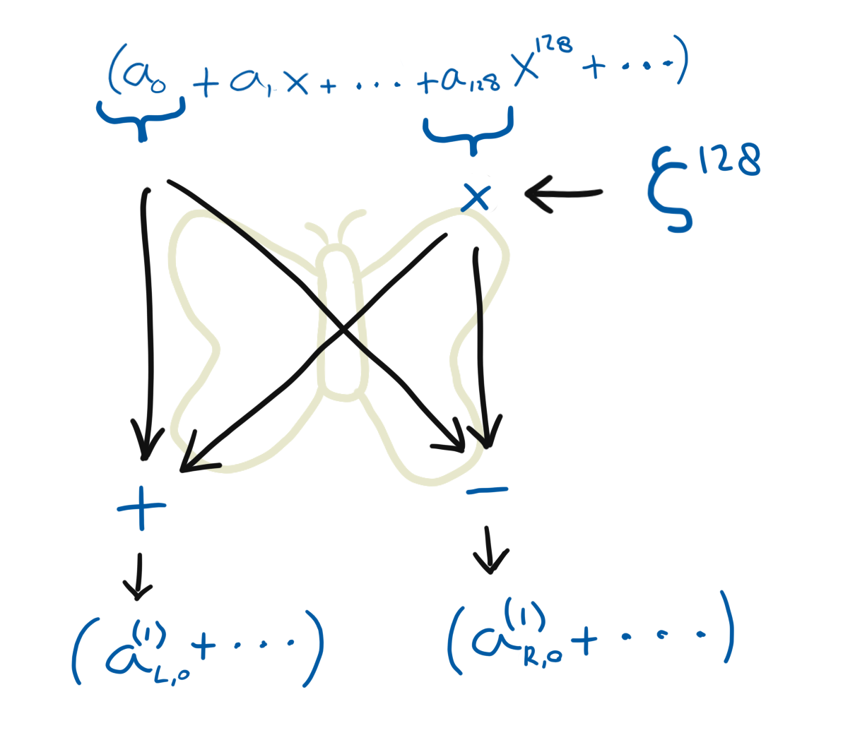
Let’s first look at \(\mathbf{a}_L^{(1)}\). We need to take all the “top” coefficients \(a_i\) where \(i \ge 128\) and reduce them modulo \((X^{128} - \zeta^{128})\). Because \(X^{128} = \zeta^{128}\), we know that \(a_iX^i = a_i\zeta^{128}X^{i - 128}\). So to get rid of the top coefficients we multiply them with \(\zeta^{128}\) and add them to the coefficient that is 128 spots further down. This results in:

\[\mathbf{a}_{L}^{(1)} = (a_0 + \zeta^{128}a_{128}) + (a_1 + \zeta^{128}a_{129})X + (a_2 + \zeta^{128}a_{130})X^2 + \ldots\]

Now let’s look at \(\mathbf{a}_R^{(1)}\). In this case the reduction polynomial has a positive \(\zeta^{128}\) term, instead of a negative one. So in this case, \(X^{128} = -\zeta^{128}\). To reduce modulo this polynomial, we would multiply with \(-\zeta^{128}\), instead of \(\zeta^{128}\):

\[\mathbf{a}_{R}^{(1)} = (a_0 - \zeta^{128}a_{128}) + (a_1 - \zeta^{128}a_{129})X + (a_2 - \zeta^{128}a_{130})X^2 + \ldots\]

A beautiful observation is that we can apply both of these formulas in parallel. Indeed, for every coefficient we only need to multiply with \(\zeta^{128}\) once, then we just respectively add and subtract, and we have done both reductions in one go!

Now we have two polynomials next to each other. The left polynomial is equal to \(\mathbf{a} \bmod{(X^{128} - \zeta^{128})}\) and the right one is \(\mathbf{a} \bmod{(X^{128} + \zeta^{128})}\).

This operation that we just have done is often called a “butterfly”, and is depicted by a “butterfly diagram”. That is because, if you squint really hard with your eyes at the diagram, you can see a butterfly in the arrows.

After the recursion from the previous section, you have probably already guessed what the next step will be.

Yup! We will again split the new polynomials in two, using the factors that we found earlier. That is, we again apply the butterfly operation on each of the (now 128) coefficients of the left polynomial \(\mathbf{a}_L\). But, instead of \(\zeta^{128}\), we now multiply in the factor \(\zeta_8 = \zeta^{64}\). For the right polynomial \(\mathbf{a}_R\) we do the same, but with the factor \(\zeta_8^3 = \zeta^{192}\). We split all of these polynomials, again and again, until we are only left with degree-0 polynomials.

---

After finishing the transformation, we can do all operations on the polynomials in a “pointwise” fashion, which has \(\mathcal{O}(n)\) complexity. To transform the polynomials, we recursed down a tree with \(\log_2 n\) “layers”, of which each did \(n\) multiplications with some \(\zeta^i\). Consequently, the complexity of the transformation is \(\mathcal{O}(n \log n)\). Hooray, we have reduced the multiplication complexity to \(\mathcal{O}(n \log n)\)!

The inverse transform ¶

Of course, the story is not finished yet. Because although we have a nice transformation to small polynomials, at some point we will have to transform them back! Fortunately, there is no need to grab another trick from our trick-box.

All the operations from the forward transform are actually pretty easily reverted. Let me explain this by looking back at the computation of the first layer in the forward transform. (In these equations, I have ditched some of the unnecessary mathematical clutter.)

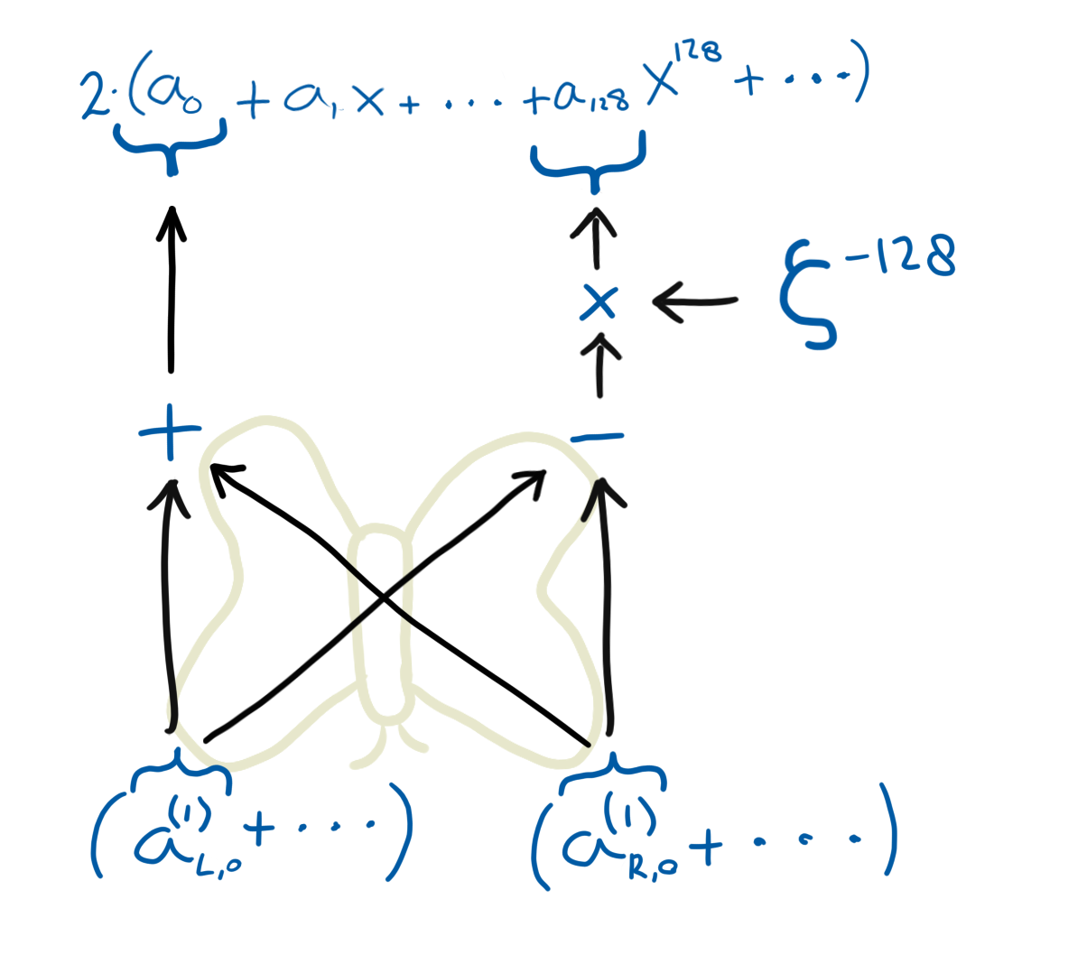
\[\begin{aligned} a_{L,0}^{(1)} &= a_0 + \zeta^{128}a_{128} \\ a_{R,0}^{(1)} &= a_0 - \zeta^{128}a_{128} \\ \end{aligned}\]

In the inverse transform, we start with \(\mathbf{a}_{L}^{(1)}\) and \(\mathbf{a}_{R}^{(1)}\) and need to get to \(\mathbf{a}\). Let’s use the equations above to find how to compute \(\mathbf{a}\). First, we take the sum of both equations:

\[\begin{aligned} a_{L,0}^{(1)} + a_{R,0}^{(1)} &= a_0 + \cancel{\zeta^{128}a_{128}} + a_0 - \cancel{\zeta^{128}a_{128}} \\ 2a_0 &= a_{L,0}^{(1)} + a_{R,0}^{(1)} \\ a_0 &= 2^{-1} \left( a_{L,0}^{(1)} + a_{R,0}^{(1)} \right) \\ \end{aligned}\]

Now take the difference of these equations:

\[\begin{aligned} a_{L,0}^{(1)} - a_{R,0}^{(1)} &= \cancel{a_0} + \zeta^{128}a_{128} - \cancel{a_0} + \zeta^{128}a_{128} \\ 2\zeta^{128}a_{128} &= a_{L,0}^{(1)} - a_{R,0}^{(1)} \\ a_{128} &= 2^{-1}\zeta^{-128} \left( a_{L,0}^{(1)} - a_{R,0}^{(1)} \right) \\ \end{aligned}\]

As you see, the reverse operation looks very similar to the forward operation. The only thing that appeared extra was an extra constant factor \(2^{-1}\). That \(2^{-1}\) factor is the same in every layer; so we can accumulate this factor for every layer into one single multiplication with \(2^{-\ell}\), where \(\ell\) is the number of layers. We will do that extra multiplication in the end of the inverse transformation (or in the beginning, it doesn’t matter).

Then we get the formulas for the inverse:

\[\begin{aligned} 2a_0 &= a_{L,0}^{(1)} + a_{R,0}^{(1)} \\ 2a_{128} &= \zeta^{-128} \left( a_{L,0}^{(1)} - a_{R,0}^{(1)} \right) \\ \end{aligned}\]

And of course, this rule also has its own diagram:

At this point, most of the “math-y” substance should be past us. The rest of this post puts this thing into context, because there is still a lot of jargon and terminology that needs to be put in context.

Let it sink in; maybe refill your coffee.

---

NTT and FFT ¶

This “transformation”, as I have been calling it all this time, that is the “number theoretic transform” (NTT). Or more specific, it is a number theoretic transform; and the one that is used in Dilithium.

One important thing to note is that the NTT is just the transformation. It does not mean the algorithm, although some of the literature is a bit stubborn about this nuance. The NTT might as well be implemented using matrix multiplication, using (for example) the formulas from Greconici’s master thesis (page 7).

Instead, the algorithm that we implemented is a reinvention of the Fast Fourier Transform algorithm (FFT), which was first invented by Gauss, but which is most often credited to Cooley and Tukey, because of their 1965 paper. Similarly, the first paper describing the inverse FFT was from Gentleman and Sande in (1966).

These papers are why most cryptographers credit Cooley–Tukey for the forward FFT algorithm and why they credit Gentleman–Sande for inverse NTT. However, while Gentleman was listed on that paper as an author, they (Gentleman) never claimed to have devised the inverse algorithm. More so, in their paper, they explicitly call it the “Sande version” of the FFT algorithm. That is because Sande invented the alternate form while following one of Tukey’s courses. Indeed, when it is credited outside of crypto, it is often credited as the “Sande–Tukey” form. Even Cooley calls it this name in their 1987 essay on the origins of the FFT algorithm.

At times, this confusion in the crypto literature seems to bother me a bit. In the natural sciences, the common names for these algorithms are just the “FFT algorithm” and the “inverse FFT algorithm” (IFFT). This is also the nomenclature that Cooley follows in their 1987 essay. I think it would be best to just stick to these names—instead of “Cooley–Tukey” and “Gentleman–Sande”—because it makes this stuff easier to follow by people that are new in the field.

Inline glossary ¶

Apart from the NTT and FFT, there are more concepts that are used in the Kyber and Dilithium NTT. This post would not be finished without a clarification of what all these terms mean. Therefore, I wrote this section as a small glossary of stuff that you might find in the specifications or in the code.

NTT

Number theoretic transform. Meaning should be clear from the rest of this post.

INTT

Inverse number theoretic transform. Inverse of the NTT.

FFT

Fast Fourier transform. Meaning should be clear from the rest of this post.

Other names for this concept:

• Decimation-in-time (DIT) algorithm
• Cooley–Tukey algorithm (CT) algorithm

IFFT

Inverse fast Fourier transform. Inverse of the FFT.

Other names for this concept:

• Decimation-in-frequency (DIF) algorithm
• Sande–Tukey (ST) algorithm
• Gentleman–Sande (GS) algorithm

NTT/FFT layer

The FFT algorithm is a recursive algorithm. A layer describes all the operations that are on the same level in the binary execution tree.

When implementors speak of merging layers, they mean that they implement the butterfly operation on two layers instead of one. This is usually done to save CPU registers or reduce branches.

(Modular) reduction

In crypto implementations you are doing arithmetic on integers all the time. While all these values should be represented modulo \(q\), that modulo operation does not happen automatically, and at some point the integers might become so large that they will overflow their registers.

A reduction step makes the numbers small again, but makes sure to preserve that they remain the same value modulo \(q\). In Kyber and Dilithium, two different reduction strategies are used: Barett reduction and Montgomery reduction.

Butterfly

Building block of the FFT and IFFT. There are two butterflies, commonly called the decimation-in-time butterfly and the decimation-in-frequency butterfly which are used in the FFT and IFFT algorithms respectively.

CRT

The Chinese remainder theorem. See dedicated section on the CRT.

\(q\)

Ring modulus. All computations are done modulo this integer. \(q = 8380417\) in Dilithium and \(q = 3329\) in Kyber. See also The structure of \(q\).

\(n\)

The polynomial length. I.e. the amount of coefficients every polynomial. In both Dilithium and Kyber \(n = 256\).

\(k\)th primitive root of unity (\(\zeta\))

The \(k\)th primitive root of unity is some number \(\zeta\), for which holds that: \[\zeta^k = 1 \pmod{q} \quad \text{and} \quad \zeta^l \ne 1 \pmod{q}, 1 \le l < k\]

In other words, if we iterate over the powers of \(\zeta\) we will have cycled back to \(1\) after exactly \(k\) steps.

In the Dilithium spec, the 512th primitive root of unity is referred to by \(r\). Its value is equal to \(r = 1753\).

In Kyber, there exists no 512th primitive root of unity. In that case, the 256th primitive root of unity is used. Its value is equal to \(\zeta = 17\).

Twiddle factor

A twiddle factor is a constant that is used in the FFT algorithm. This term was coined by Sande in 1966. A twiddle factor is always a power of the primitive root of unity.

NTT domain/frequency domain

The NTT domain or frequency domain is the domain where values are stored after they are transformed with the NTT.

Because the FFT algorithm has mainly been used to transform time-series data to frequency-spectrums, it is common to say that the input to the FFT algorithm is provided in the time domain, and the output is given in the frequency domain.

Time domain

The “regular” domain, where no NTT has been applied (yet).

Because the FFT algorithm has mainly been used to transform time-series data to frequency-spectrums, it is common to say that the input to the FFT algorithm is provided in the time domain, and the output is given in the frequency domain.

Circular/cyclic convolution

The convolution of two periodic sequences. If we take each of the numbers in these sequences, and use them as coefficients of some polynomials \(\mathbf{a},\mathbf{b} \in \mathbb{Z}_q[X]/(X^n - 1)\), then computing the circular convolution of these sequences is the same as computing \(\mathbf{a} \cdot \mathbf{b}\).

Negacyclic convolution

The nega-cylic convolution is similar to the cyclic convolution, but the reduction polynomial of the ring is \(X^n + 1\) instead of \(X^n - 1\). In other words: if we take the numbers in two sequences, and use them as coefficients of some polynomials \(\mathbf{a},\mathbf{b} \in \mathbb{Z}_q[X]/(X^n + 1)\), then computing the negacyclic convolution of those sequences is the same as computing \(\mathbf{a} \cdot \mathbf{b}\).

The whole point of Dilithium and Kyber is that the negacyclic convolution can be computed cheaply using \(\mathrm{NTT}^{-1}(\mathrm{NTT}(\mathbf{a}) * \mathrm{NTT}(\mathbf{b}))\), where \(*\) denotes pointwise multiplication.

The structure of \(q\) in Kyber ¶

Before I end this post (cause it’s been going for way too long now), I should explain one last thing: the structure of \(q\). The point is that earlier in this post, I just assumed that a \(k\)th primitive root of unity would exist if we needed one. If you think about it, it becomes obvious that that might not always be the case. In Dilithium, we’re good, because there indeed exists a 512th primitive root of unity mod \(q\). However in Kyber (version 2), that is not the case, as there only exists up to a 256th primitive root of unity mod \(q\).

This poses a problem in the factorization of the Kyber ring. In Kyber, we cannot factor the reduction polynomial down to degree-0 polynomials; we can only go down to degree-1.

As a consequence, Kyber’s NTT algorithm has only 7 layers and it produces degree-1 polynomials. Therefore, the “pointwise multiplication” in Kyber is not really pointwise, and the “pointwise multiplication” in Kyber is still a bit complicated.

---

Epilogue ¶

That was quite a long stretch. When I started writing this, I didn’t actually expect to produce a blog post that is as long as this one.

I hope that this post could have been of use to you. Feel free to ask questions or provide feedback by dropping me an email.

Acknowledgements ¶

Thanks to Bas for taking the time to explain the NTT construction to me multiple times; and Bas and Marrit for proofreading this post before I put it online.